What is a pattern and why does it matter for AI-enabled operational excellence?

Key Takeaways:
- Patterns let us use part of the picture to see things that are otherwise hidden. Interesting events are often visible only after the fact: we frequently lack the means of seeing interesting events as they unfold.
- Descriptive statistics and regressions on real-time data reveal patterns that can be used to infer simple hidden behaviors.
- We need the ability to work with more complex, multivariate patterns in real-time data so that we can surface higher value behaviors.
- In this article we discuss an approach to inferring such complex hidden behaviors that is widely applicable across a range of use cases without modification.
Pattern [pa-tərn]: a reliable sample of traits, acts, tendencies, or other observable characteristics.
Patterns let us infer a broader set of behaviors from a sample of those behaviors: when I observe this, this and this, that is likely to happen next. They let us infer what might be happening without having access to the entire picture. We see patterns and understand the world in terms of patterns because information is never perfect yet we must make decisions quickly from this imperfect information.
Patterns can be simple or complex, univariate or multivariate. Simple, univariate patterns often help us make sense of simple situations. For example, the increasing volume of someone’s voice as you start to lean towards a broken railing is a clear call for caution. Complex situations often require multivariate pattern analysis. That is, they require interpretation of far more complex patterns, spanning multiple signals, that can easily overwhelm human cognition. For example in a plant running a mix of different products, what combinations of equipment behavior and input material quality indicate that a process chamber is wearing out faster than expected and will require early reconditioning? Traditional methods over-simplify the signals, effectively throwing out what we cannot easily interpret. But for many interesting situations, the signal is buried in this “noise.” We need a better way of extracting and summarizing so that the hidden signal can be used – we need a better way to create patterns that capture the irregular, multi-component, finely detailed nature of the most interesting events.
Let’s talk about various types of hidden behaviors, ways of finding them in real-time data, and how those patterns can be leveraged for predictive operations. Let us consider a compressor. The compressor has periodic seal failures which we want to avoid. We have no direct measurement of the seal’s health. That is hidden information. We do have continuous information from numerous sensors within the compressor (e.g. discharge pressure, suction flow rate, differential pressures, etc.) from which to infer the operational state of the compressor seal.
Descriptive Statistics Approach
One way to look at the compressor is to use descriptive statistics. This approach summarizes the time series data into static pictures. It is the realm of things like averages, standard deviations, rates of change and so forth.
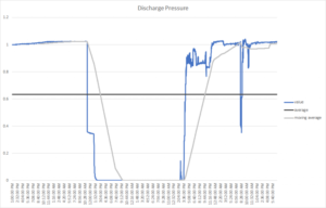
Fig 1 – The behavior of the discharge pressure of a compressor is shown in blue. There are multiple behaviors of potential interest (e.g. a shutdown, a start-up transient and a pressure drop spike). The statistical summaries (greys) lose much of the interesting behavior. A simple average (dark grey) misses all of the behaviors. The moving average (light grey) catches the shutdown but misses the start-up transient and pressure spike.
Using this approach, we might be able to see that the average discharge pressure is X and that it has a variance of Y. We could do this for each of the sensors and ascertain the relationship between each descriptive measure and the occurrence of a seal failure. This quickly becomes overwhelming and often produces poor sensitivity and specificity of the failure. It is also difficult to capture the dynamics of a changing system using the static pictures that descriptive statistics provide, especially one that has many interacting components like in the compressor. While this approach is simple to implement, and indeed forms an important part of statistical process control (SPC), it is not well suited for dealing with problems like prediction. In predictive cases, the pattern indicating failure is often more subtle than an average shift can detect or is multivariate in nature. In other words, it is more complex than a single sensor can reliably capture, requiring a multivariate pattern analysis approach.
Regression Analysis Approach
Another way to approach the seal failure prediction case is via regression analysis. This approach attempts to fit a line or curve to the sensor data, either singly (univariate) or using groups of sensors (multivariate). By plotting this function over the life of a part, a threshold value is found which corresponds with failure. When new sensor data is fed into the function, it generates a value. When that value passes the threshold, it is likely that failure has occurred. By projecting the current value to the threshold value, it is possible to estimate the time to failure (TTF).
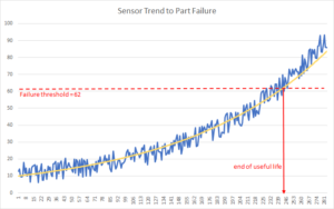
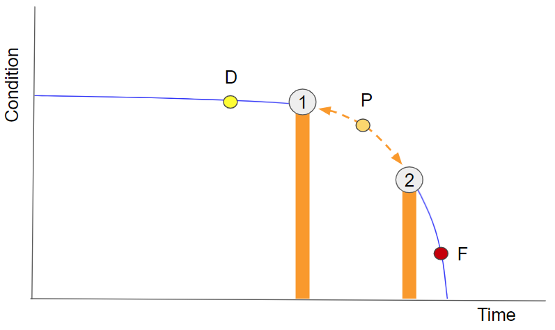
Fig 2 – Historical data can be fed into a multivariate model (blue line) to identify a threshold (red dashed line) where the part reaches its end of useful life.
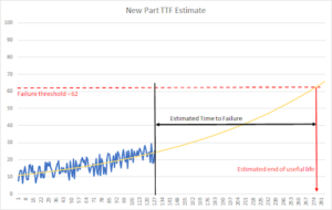
Fig 3 – New data is collected and fed into the multivariate model (blue). As the part ages, a fit to the multivariate model can be made (yellow). The projection of the fit to the threshold value (red) provides an estimated time to failure (black line).
This can be a powerful technique when behaviors change smoothly over time. However, not all cases are like this. Often the pattern of operation varies significantly from day to day and the noise from these changes can mask trends within the data. Other times the failure is sudden, not preceded by a smoothly trending change. We have seen cases where the trend is only reliable a short period before the failure. In such instances another method is needed to identify the point in time after which the trending approach can work, necessitating a hybrid approach. In the compressor case, operations varied significantly over time so that a trend based on earlier operation was not applicable to later operation. The pattern of failure was there but was not discernible as a trend.
Feature Engineering and Classification Approach
We have found that a combination of feature engineering and classification provides a more flexible way to describe the time variant behaviors of the system. In this multivariate pattern analysis approach, the “shape” of the sensor data as it changes in time is encoded in a form that lets a classification algorithm distinguish between those “shapes.” These shapes, taken across all sensors, form the patterns. Using machine learning techniques, these patterns are then matched to specific behaviors of interest such as a part failure or the behavior which precedes a part failure.
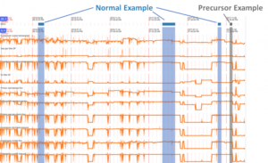
Fig 4 – The raw time series sensor data is shown in orange for a number of compressor sensors. The user is able to mark certain periods of operation as normal (dark bluehorizontal bars) or as precursor to seal failure (grey horizontal bar). The colored columns represent the data that Falkonry will use to represent each condition (normal or precursor).
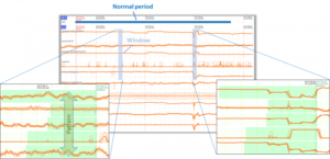
Fig 5 – Zooming in shows the details of a “normal” period. Falkonry breaks up each period into multiple windows. Two window examples are shown as tall vertical blue boxes. From each window Falkonry’s multivariate pattern analysis constructs a single pattern using the shapes of the most important sensor traces within it (light green boxes). All the patterns in the normal period are taken together to define the “normal” classification.
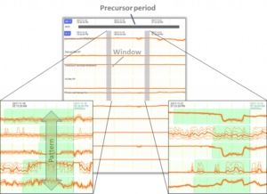
Fig 6 – Zooming in shows the details of the “precursor” period. Falkonry breaks up each period into multiple windows. Two window examples are shown as tall vertical greyboxes. From each window Falkonry’s multivariate pattern analysis constructs a single pattern using the shapes of the most important sensor traces within it (light green boxes). All the patterns in the precursor period are taken together to define the “precursor” classification.
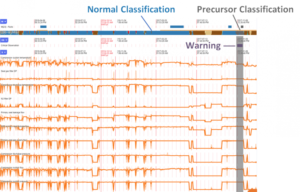
Fig 7 – Using these patterns, Falkonry software classifies the remainder of the time series data into normal (blue), precursor (grey), unclassified (brown) and unknown (red). As can be seen, the precursor classification (grey vertical bar) fully captures the warning event (purple). This means that Falkonry’s multivariate pattern analysis system was able to correctly predict the seal failure while also correctly classifying the other normal operational states of the compressor.
In the example shown in the figures above, the difference between normal and precursor patterns is not obvious to the human eye. There is no clear threshold or trend which corresponds to the warning period, yet the warning pattern Falkonry sees is distinct. This is the power of a time series pattern.
This approach allows a much more dynamic picture of the system to emerge. Patterns of behavior which are fine grained or which do not smoothly change over time can be captured using this approach. It fits with one’s intuitive understanding of patterns – when I see this, I can expect that. Because it is based on that generalized method of observation, it can also be applied to a wide range of conditions beyond those which descriptive statistics or regression approaches can accommodate.
The Falkonry Way
Feature engineering is not a solved problem, especially for time series data: this is hard to do. We have found a way that has proven robust, sensitive and applicable across industries and use cases without modification. This makes it easy enough for plant engineers to take advantage of, allowing them to perform powerful multivariate pattern analysis based ML predictions as part of their day-to-day work.